Demystifying Linear Optimization: Squeeze Out Higher Profits Without Squeezing Your Company
Deciding how best to use limited resources is a universal issue that spares no individual or business. In today’s competitive quarter-to quarter environment, it’s critically important to your company’s profitability (and longevity) that its people and assets are used most efficiently. While this is an obvious truism, it is not always obvious how to go about doing this—especially when dealing with complicated networks.
The companies going from “good” to “great” arrive at the right answers when it comes to making business decisions on product mix, logistical routing and demand planning through a process commonly known as linear programming (tabbed “linear” because the maximized or minimized answers are assumed to be linear in nature). This mathematical exercise squeezes profitability to the closest dollar while considering constraints of the business—limitations such as radius of delivery, fleet size, manufacturing capacity, amount of material, lead times, space, etc. When done correctly, the business can rest easy knowing there is not significant value being left on the table. However, many companies shy away from the technology because they just don’t understand it.
The purpose of this article is to demystify the complexity behind optimization by illustrating how it works in a case study context.
The Situation
The North American division of a global manufacturer was becoming progressively more capacity-constrained due to bottlenecks in its distribution network, while product demand in key regional markets was growing in disproportion to the regional plant’s ability to supply. The CEO made it a key priority to address this in order to increase profitability. However, due to the complexity of the distribution network and trade-offs between economic drivers, it was not a simple “back-of-the-envelope” exercise to quantify the opportunity and other costs of these bottlenecks. Assessing the overall impact of potential options was also very difficult.
In response, a project team composed of internal and external supply chain professionals used a framework to help the company’s executives refine the strategies for upcoming growth without hurting current customer obligations. The project’s objectives were threefold:
- Identify and value strategic network opportunities.
- Maximize operational profits.
- Provide visibility on future month-by month system constraints (e.g., material shortages, railcar availability, silo capacity).
The results of the project were phenomenal. The team confidently recommended:
- A rebalancing of product to 25 markets (without sacrificing sales) in order to ensure greatest overall profit margin.
- Tactical distribution moves to save over 5% in freight and other variable costs.
- Payback analysis on the exact benefits of resolving the top network constraints.
- A forecasting tool to measure profitability and network impact of future greenfield locations.
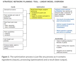
Network optimization is commonplace in most logistics-based industries and is not inherently difficult to execute, provided some basic understandings of the fundamentals are in place. With any optimization exercise, there are three parts: inputs, the process and the output (Figure 1). In this case the company wanted the output to reflect maximized profits (not necessarily just minimized costs.)
The Constraints (aka inputs)
First, the rules of the game must be established in the form of operating constraints, which form the “dimensions of the field” that the solver will ultimately play in. Demand is viewed as a constraint to a linear program (LP) since a location can only be given so much product before it exceeds its ability to convert the product into sales. In the client’s case, the company had 25 sales locations to consider, each with varying demand for the same product.
Another sideline to the field included margin information so that output would be based on overall profit. Specifically, this information detailed the individual product, fixed and delivery costs.
Finally, the capabilities of the network were entered, from plant manufacturing rates to railcar and truck capabilities.
With these rules in place, the team went to work ensuring they could replicate the previous year’s operational performance and thus establish a trustworthy baseline.
The Processing (aka linear optimization)
An optimized solution merely means it is the “best use” of limited resources available. The “best use” usually means something positive (like efficiency or profit) is maximized or things to be avoided (like costs) are minimized. A quick breakdown of what happens during a linear optimization is illustrated in the example below:
Imagine an operation that wants to minimize the costs of meeting sales demand. The available finished product storage capacity in its region is 200 tons between two neighboring manufacturing plants. The only thing preventing infinite production (so far) is how many products could go into each storage silo. Graphically stated on an x and y axis, that scenario is displayed by the blue line in Figure 2. The area under that curve represents all the product they can make (Plant 1 + Plant 2 = 200 tons in total.)
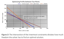
Now, making the example a bit more realistic, we add other operational constraints that cut into what the plants can produce: the supply of raw materials and the amount of available labor. When these constraints are likewise graphed, they cut into the wide open area under the blue line. As more and more limitations are introduced, the area under the curve becomes smaller and smaller.
Here’s where the solver mechanism adds value: The point of intersection of the innermost constraint lines (which in this case are blue and orange) indicates the optimum amount of tons to produce from each plant (Plant 1= 120; Plant 2= 80) while playing by the rules of the limits.
The LP takes into account the absolute limits on demand, production capacity, delivery trucks, etc., but is also allowed to play with those variables in an adjustable fashion—within the stated thresholds. The solver is merely trying to find the point where all most limiting constraints intersect while allowing for the greatest area under the curve (i.e. maximizing profit). Within a minute, the solving mechanism whips through hundreds of thousands of iterations and sorts through 13,000 adjustable variables until it is sure it has found the best solution. Now it’s time to analyze the output.
The Output
One of the best things about a computer program is that it will do what you say. And sometimes, one of the worst things about a program is that it will… do what you say. The LP is quite literal; it does exactly as we say and not as we mean. So therefore, analyzing the answer to understand the nature of the underpinning moves is essential in this final phase.
As diligent as we intend to be on the front end, it is very easy to overlook an obvious constraint—which can wreak havoc on the answer. For example, a plant might find it very cost-effective to make product and then keep it all to itself in order to minimize shipping costs—unless constraints are in place to make this a very unattractive (or impossible) option. This phase may take a few runs to ensure the model is error-proofed.
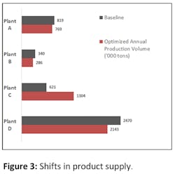
So what picture emerged from the abyss? The most profitable, optimized scenario shows a significant shift in manufacturing sourcing to Plant C at the expense of Plants A, B and D (Figure 3). These sourcing shifts are motivated from the identification of more efficient distribution modes in Markets 1-6 (Figure 4).
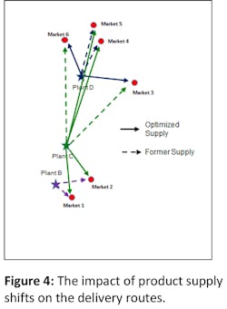
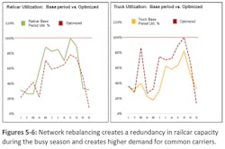
The largest swing is in Market 3, with Plant C trading nearly 70% of its market volume to Plant D. These moves translate to a savings of $2.1 million in this one region (while still meeting customer requirements). And from a logistics standpoint, one can see the forecasted shift in transport needs during September-October from rail to truck (Figures 5-6). This shift effectively allows the company to roll off excess railcar leases and switch to the more variable delivery cost in trucks.
Network Debottlenecking
Every process has a limiting factor—such as market demand, funds, equipment capacity, time, etc.—that prevents perpetual flow. And not all bottlenecks are created equal. Some may have no value since they are captive to something more critical, while others are undoubtedly costing the enterprise in sales or excess labor. How does one know which ones are worth resolving and the respective paybacks? Networks are not unlike the timeless Rubik’s Cube toy—dynamic and intertwined—and figuring out the overall impacts of knocking down a bottleneck is something easily accomplished with a program like this one.
The team was able to view processes in the network that were “maxed out” (or at 100%) by setting up output tables derived directly from the results of the LP. As the example shows in Figure 7, Plant B was potentially holding up the works as it was forecasted to be loading product on trucks and railcars May through October 24 hours a day.
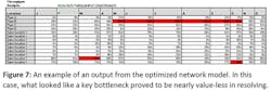
Though there are more technical ways to measure the bottleneck’s value and significance, the team found it was a relatively simple exercise to incrementally raise the throughput level at Plant B in the model and study the changes in overall profit return. In this case, there was no significant return since there were other limiting constraints in the downstream storage capacities. When the storage capacity issue was isolated and “fixed” in the model, the result was like unclogging a drain: volume flowed much easier. Without network modeling ability, it would have been very difficult to quantify these critical bottlenecks and their accompanying values.
The problems faced by decision makers in today’s competitive, fast-paced environment are often extremely complex and can be addressed in a myriad of ways. Using models in decision-making and problem-solving is really not new and is certainly not just tied to computers and spreadsheets. Quite frequently a mental model is enough to analyze a problem and go forward. But for complex business decisions, it may be impossible to capture all the moving parts without using a tool like an LP.
One of the chief benefits from network modeling is the ability to test decisions that would have been otherwise impossible to do in reality. Furthermore, linear programs don’t require much bandwidth from the organization to develop and run. The biggest lesson for this logistics company? Just because the problem is thorny and complex does not mean the answer has to be.
Ryan Brown is the founding consultant at Next Level Essentials LLC, a profit improvement practice for the construction materials industry.